The Basic Reed
Woodwind
Reed woodwinds include
saxophones, clarinets, oboes, and bassoons.
Other reed instruments include harmonicas, accordions, and some organ
pipes. These pages will concentrate on
monophonic instruments, like saxophones.
Our discussion will assume
some familiarity with the blown pipe model.
In fact, we’ll borrow some pieces of it.
Reed woodwinds can have two
kinds of reeds: a single reed, as used
in a clarinet or saxophone, or a double reed, as used in an oboe or
bassoon. Since I can’t find a
double-reed model, we’ll model a single reed, and then use EQ to attempt to
mimic oboes and bassoons.
Reed woodwinds can have two
kinds of bores: a cylindrical bore, as
used in a clarinet, or a conical bore, as used in saxophones, oboes, and
bassoons. Our bore will be able to
simulate both kinds of bores.
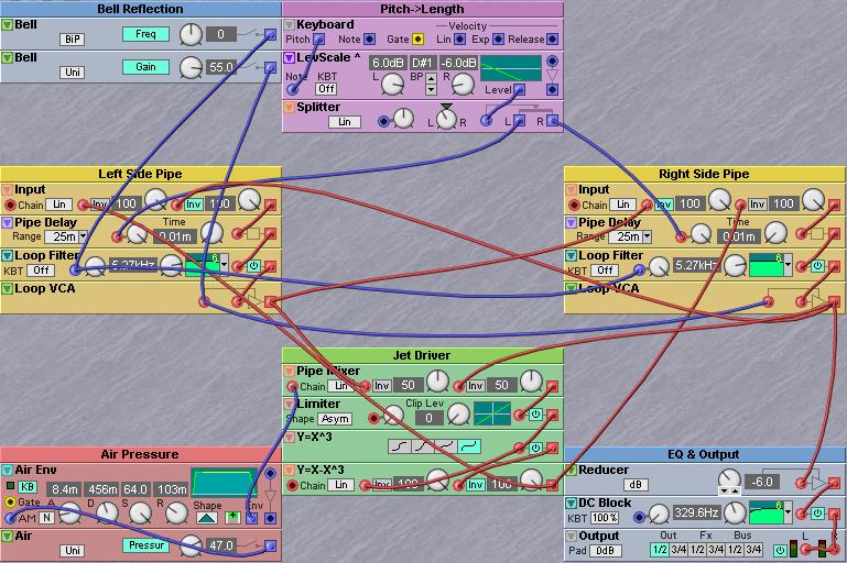
The basic model
The basic model is
below. It doesn’t sound like much yet,
but don’t be discouraged. There are many
improvements to be made.
How does it work?
The operation is similar to
our blown pipe. Once again, the
combination of the jet driver and a tuned delay is the basis of the model. In fact, the jet driver is identical to the
one in the blown pipe model.
It’s the delay line that’s
different. In fact, there are two
delays, one each in the Left Side Pipe and Right Side Pipe.
Let’s trace the signal
flow. We’ll begin with the Left Side
Pipe. This section contains a delay
line, a lowpass filter, and a gain control.
The output then goes to the Right Side Pipe, and is inverted as it
enters. The Right Side Pipe is identical. It contains another delay line, a lowpass
filter, and a gain control. The output
then returns to the Left Side Pipe, and is again inverted as it enters. Notice that the lowpass filters and gain
controls have matching characteristics, but that the delay lines can have
different lengths.
It turns out that this loop
is, in fact, the standard physical model of a string. One delay represents the length of string
from the pick to the bridge, and the other delay represents the length of
string from the pick to the nut. The
lowpass filters and inverting gain controls represent the reflections and
energy losses at the bridge and nut.
But instead of “plucking”
the string by injecting a noise pulse into it, we’ve placed a jet driver at the
pick point. We’ve summed the outputs of
the delays, divided them in half, and then added them to the input air
pressure. This feeds the jet
driver. The output of the jet driver
goes back into both delay lines. This
kind of model is called a “blown string”.
It’s an attempt to model a conical bore in an inexpensive way.
Cylindrical and conical bores
It’s the cylindrical bore of
a clarinet that gives it that “woody” sound.
This is because the straight bore supports only odd harmonics (more or
less). The conical bores of saxophones,
oboes, and bassoons are the reason that their sounds include even harmonics.
There are two common ways to
model conical bores. The “physical” way
is to create something called a Kelly-Lochbaum filter, containing dozens of
tiny delay lines, adders, and multipliers.
Using this method, any shape of bore can be created.
We don’t have a
Kelly-Lochbaum module in the G2, so we’ll use the “non-physical” way: the blown
string. It can’t do everything a
Kelly-Lochbaum filter can do, but it’s enough to create even harmonics, and we
can do the rest with EQ.
We’ll control the “shape” of
our bore by controlling the ratio of the delay line lengths, via the Pan knob
on the “Splitter” Pan module. If the
knob is in the center, the two lengths are equal, and our pipe sounds woody,
like a clarinet. But if one length is
longer than the other, the sound begins to include even harmonics. Varying this control is a lot like varying
the pulse width of a pulse-wave oscillator.
Regardless of the position of the Pan knob, the total length of the loop remains the same, and this is why the
pitch doesn’t change when the Pan knob is moved.
The delays are tuned using
an old trick from the original Nord Modular: the Level Scaler Module. This module can be linked to the keyboard and
adjusted to output a -6dB/octave slope.
Since -6dB represents a 50% reduction, and since we want the delay line
to become 50% shorter with each increasing octave, this module is perfect for
the task.
The control parameters
This model has 5 control
parameters. They are:
- Pitch. Pitch
should be directed to the Note input of the Level Scaler. In this patch, the pitch comes directly
from the keyboard.
- Pipe
Shape. The shape of the pipe is controlled by
the position of the Pan module labeled Splitter. Pipe shape can be modulated via the modulation
input on the Splitter.
- Air
Pressure. This drives the model, and represents
the air coming from the player’s lungs.
Air pressure should be directed to the Chain input of the Pipe
Mixer module. This is typically
provided by an envelope generator, or a breath controller.